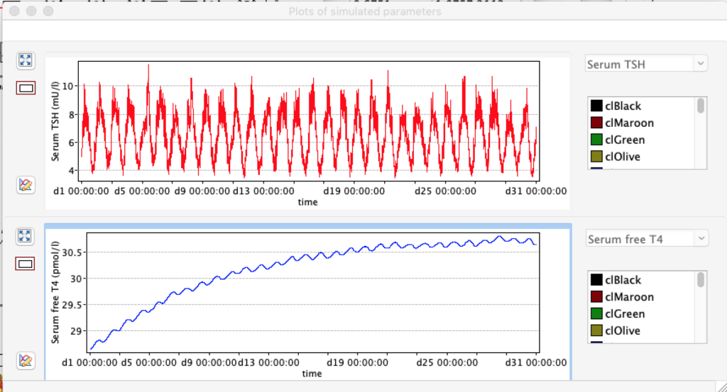
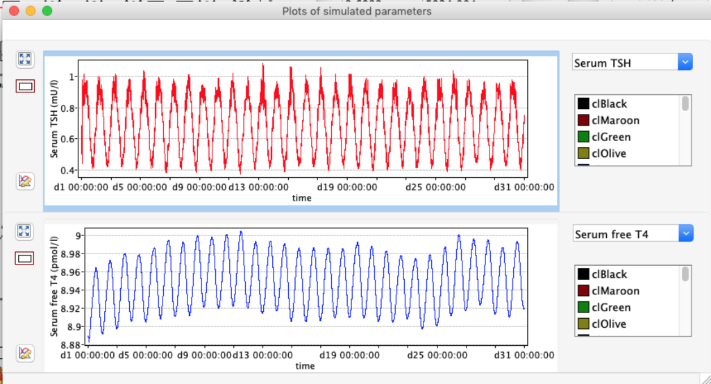
TSH variation in 24 hours
Exploring this modelscenario – SimThyr?
Method importing libraries:
library(readr)
library(dplyr)
library(tidyr)
library(tidyverse)
library(WVPlots)
library(ggridges)
library(magrittr)
library(ggplot2)
library(clinfun)
library(e1071) #kurtosis
library(SPINA)
Dataset 1: SimThyr – SimThyr 4.0
The versatile thyroid simulator for education and research. (Ref: SimThyr, RRID:SCR_014351. http://scicrunch.org/browse/resources/SCR_014351. The Digital Object Identifier (DOI) for SimThyr is 10.5281/zenodo.1303822. Project page: https://simthyr.sourceforge.io/index.html)
In this SimThyr simulation 50 days and the standard setting is used. In “preferences” only hours is used. This is due the visualisation model – (WVPlots::ScatterHistN – https://winvector.github.io/WVPlots/articles/WVPlots_examples.html – the action behind is described here: https://github.com/WinVector/WVPlots/blob/main/R/ScatterHistC.R (Note ScatterHistN is at the buttom of the document)) – can’t handle characters (yet?)
Dataset import, tidying and calculations:
CSVdotcsv <- read_csv("http://www.glensbo.dk/Files/Timer50StandardCSV.csv",
col_names = TRUE,
skip_empty_rows = TRUE,
col_types = "-ddddddddd-")%>% slice(-1)
## Warning: Missing column names filled in: 'X11' [11]
## Warning: 9 parsing failures.
## row col expected actual file
## 1 t a double day h:m:s 'http://www.glensbo.dk/Files/Timer50StandardCSV.csv'
## 1 TRH a double ng/l 'http://www.glensbo.dk/Files/Timer50StandardCSV.csv'
## 1 pTSH a double mU/l 'http://www.glensbo.dk/Files/Timer50StandardCSV.csv'
## 1 TSH a double mU/l 'http://www.glensbo.dk/Files/Timer50StandardCSV.csv'
## 1 TT4 a double nmol/l 'http://www.glensbo.dk/Files/Timer50StandardCSV.csv'
## ... .... ........ ......... ....................................................
## See problems(...) for more details.
Additional calculations and add columns via mutate. The solution for me (as this long string of mutations made problems in the .Rmd file) was to mutate to CSVdotcsv and assign the result to CSVdotcsv. (Tips from Practical Data Science With R, https://livebook.manning.com/book/practical-data-science-with-r-second-edition/chapter-2/v-6/comment-501826)
CSVdotcsv <- CSVdotcsv %>%
mutate_if(is.character,as.numeric)%>%
mutate(ratio = FT3/FT4,
TSH_Sum = (FT4*0.52)+(FT3*0.38)+((FT4+FT3)*0.1),
TSH_TSH_Sum = TSH/TSH_Sum,
SPINA_GT = SPINA.GT(CSVdotcsv$TSH, CSVdotcsv$FT4),
SPINA_GD = SPINA.GD(CSVdotcsv$FT4, CSVdotcsv$FT3),
TSHI = estimated.TSHI(CSVdotcsv$TSH, CSVdotcsv$FT4),
TRH_TSH = TRH/TSH,
TT4_FT4 = TT4/FT4,
TT3_FT3 = TT3/FT3)
*
I have used col_types = “cd…..” because this is a uniform dataset I use a lot. It makes it easy to change the format of/ -delete the columns if needed
+
slice(-1) deletes the second row which contains additional headers not necessary for the calculations in these plots. (See warning above)
+
the new columns for calculations (/the slash is not accepted in the header)
+
Below is a str() and summary()
str(CSVdotcsv)
## tibble [43,201 × 18] (S3: spec_tbl_df/tbl_df/tbl/data.frame)
## $ t : num [1:43201] 0 0 0 0 0 0 0 0 0 0 ...
## $ TRH : num [1:43201] 2500 3221 1152 2193 778 ...
## $ pTSH : num [1:43201] 4 4 4 4 4 4 4 4 4 4 ...
## $ TSH : num [1:43201] 1.81 1.81 1.8 1.77 1.75 ...
## $ TT4 : num [1:43201] 122 122 122 122 122 ...
## $ FT4 : num [1:43201] 17.7 17.7 17.7 17.7 17.7 ...
## $ TT3 : num [1:43201] 3.22 3.22 3.22 3.22 3.22 ...
## $ FT3 : num [1:43201] 5.35 5.35 5.35 5.35 5.35 ...
## $ cT3 : num [1:43201] 11694 11694 11694 11694 11694 ...
## $ ratio : num [1:43201] 0.303 0.303 0.303 0.303 0.303 ...
## $ TSH_Sum : num [1:43201] 13.5 13.5 13.5 13.5 13.5 ...
## $ TSH_TSH_Sum: num [1:43201] 0.134 0.134 0.133 0.131 0.13 ...
## $ SPINA_GT : num [1:43201] 3.37 3.37 3.39 3.42 3.45 ...
## $ SPINA_GD : num [1:43201] 28 28 28 28 28 ...
## $ TSHI : num [1:43201] 2.97 2.97 2.97 2.95 2.94 ...
## $ TRH_TSH : num [1:43201] 1378 1776 639 1237 444 ...
## $ TT4_FT4 : num [1:43201] 6.9 6.9 6.9 6.9 6.9 ...
## $ TT3_FT3 : num [1:43201] 0.601 0.601 0.601 0.601 0.601 ...
## - attr(*, "problems")= tibble [9 × 5] (S3: tbl_df/tbl/data.frame)
## ..$ row : int [1:9] 1 1 1 1 1 1 1 1 1
## ..$ col : chr [1:9] "t" "TRH" "pTSH" "TSH" ...
## ..$ expected: chr [1:9] "a double" "a double" "a double" "a double" ...
## ..$ actual : chr [1:9] "day h:m:s" "ng/l" "mU/l" "mU/l" ...
## ..$ file : chr [1:9] "'http://www.glensbo.dk/Files/Timer50StandardCSV.csv'" "'http://www.glensbo.dk/Files/Timer50StandardCSV.csv'" "'http://www.glensbo.dk/Files/Timer50StandardCSV.csv'" "'http://www.glensbo.dk/Files/Timer50StandardCSV.csv'" ...
## - attr(*, "spec")=
## .. cols(
## .. i = col_skip(),
## .. t = col_double(),
## .. TRH = col_double(),
## .. pTSH = col_double(),
## .. TSH = col_double(),
## .. TT4 = col_double(),
## .. FT4 = col_double(),
## .. TT3 = col_double(),
## .. FT3 = col_double(),
## .. cT3 = col_double(),
## .. X11 = col_skip()
## .. )
summary(CSVdotcsv)
## t TRH pTSH TSH TT4
## Min. : 0.0 Min. : 0.25 Min. : 0.0002 Min. :1.081 Min. :121.9
## 1st Qu.: 5.0 1st Qu.: 1222.85 1st Qu.: 0.9798 1st Qu.:1.562 1st Qu.:127.0
## Median :11.0 Median : 2124.75 Median : 1.6931 Median :2.076 Median :127.8
## Mean :11.5 Mean : 2519.40 Mean : 2.1751 Mean :2.036 Mean :127.2
## 3rd Qu.:17.0 3rd Qu.: 3535.33 3rd Qu.: 2.7899 3rd Qu.:2.471 3rd Qu.:128.2
## Max. :23.0 Max. :11181.38 Max. :24.7769 Max. :3.479 Max. :128.8
## FT4 TT3 FT3 cT3 ratio
## Min. :17.66 Min. :3.216 Min. :5.351 Min. :11691 Min. :0.2998
## 1st Qu.:18.40 1st Qu.:3.345 1st Qu.:5.565 1st Qu.:12166 1st Qu.:0.3018
## Median :18.52 Median :3.374 Median :5.614 Median :12244 Median :0.3024
## Mean :18.44 Mean :3.351 Mean :5.575 Mean :12192 Mean :0.3024
## 3rd Qu.:18.57 3rd Qu.:3.378 3rd Qu.:5.621 3rd Qu.:12281 3rd Qu.:0.3031
## Max. :18.66 Max. :3.385 Max. :5.632 Max. :12337 Max. :0.3041
## TSH_Sum TSH_TSH_Sum SPINA_GT SPINA_GD TSHI
## Min. :13.52 Min. :0.07605 Min. :2.422 Min. :27.72 Min. :2.527
## 1st Qu.:14.08 1st Qu.:0.11061 1st Qu.:2.960 1st Qu.:27.91 1st Qu.:2.924
## Median :14.18 Median :0.14711 Median :3.255 Median :27.96 Median :3.208
## Mean :14.11 Mean :0.14432 Mean :3.424 Mean :27.96 Mean :3.158
## 3rd Qu.:14.21 3rd Qu.:0.17504 3rd Qu.:3.866 3rd Qu.:28.03 3rd Qu.:3.386
## Max. :14.27 Max. :0.25539 Max. :4.994 Max. :28.12 Max. :3.713
## TRH_TSH TT4_FT4 TT3_FT3
## Min. : 0.125 Min. :6.901 Min. :0.601
## 1st Qu.: 715.948 1st Qu.:6.901 1st Qu.:0.601
## Median :1117.158 Median :6.901 Median :0.601
## Mean :1186.705 Mean :6.901 Mean :0.601
## 3rd Qu.:1583.254 3rd Qu.:6.901 3rd Qu.:0.601
## Max. :4519.021 Max. :6.901 Max. :0.601
Result:
From this scatterplot you can see TSH varies a lot during 24 hours (reflecting the diurnal nature of TSH). For each hour the number of readings reflects pooled data from 50 days.Likevise the data show higher TSH in the late night and early morning and opposite trend afternoon and evening.Consequences for blood sampling? Another observation is these two TSH values are skeewed – either left or right.
*
50 days 24h
kurtosis(CSVdotcsv$TSH) # -1.209175
+
50 days from 00:00 to 07:00
kurtosis(CSV_subset_0_7$TSH) #0.1163531
+
50 days from 08:00 to 15:00
kurtosis(CSV_subset_8_15$TSH) #-1.056109
+
50 days from 16:00 to 24.00
kurtosis(CSV_subset_16_24$TSH) #-0.4848253
+
50 days only 08:00
kurtosis(CSV_subset$TSH) #-0.2717369 only numbers from 8.00?????
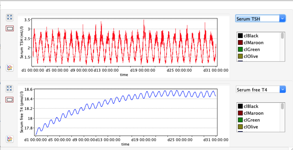
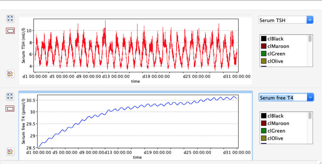
FIG. 1

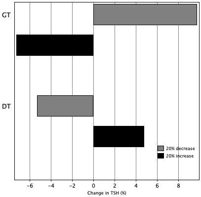
For TSH you see an interesing pattern with a clear shift during the day.
summary(CSVdotcsv)
## t TRH pTSH TSH TT4
## Min. : 0.0 Min. : 0.25 Min. : 0.0002 Min. :1.081 Min. :121.9
## 1st Qu.: 5.0 1st Qu.: 1222.85 1st Qu.: 0.9798 1st Qu.:1.562 1st Qu.:127.0
## Median :11.0 Median : 2124.75 Median : 1.6931 Median :2.076 Median :127.8
## Mean :11.5 Mean : 2519.40 Mean : 2.1751 Mean :2.036 Mean :127.2
## 3rd Qu.:17.0 3rd Qu.: 3535.33 3rd Qu.: 2.7899 3rd Qu.:2.471 3rd Qu.:128.2
## Max. :23.0 Max. :11181.38 Max. :24.7769 Max. :3.479 Max. :128.8
## FT4 TT3 FT3 cT3 ratio
## Min. :17.66 Min. :3.216 Min. :5.351 Min. :11691 Min. :0.2998
## 1st Qu.:18.40 1st Qu.:3.345 1st Qu.:5.565 1st Qu.:12166 1st Qu.:0.3018
## Median :18.52 Median :3.374 Median :5.614 Median :12244 Median :0.3024
## Mean :18.44 Mean :3.351 Mean :5.575 Mean :12192 Mean :0.3024
## 3rd Qu.:18.57 3rd Qu.:3.378 3rd Qu.:5.621 3rd Qu.:12281 3rd Qu.:0.3031
## Max. :18.66 Max. :3.385 Max. :5.632 Max. :12337 Max. :0.3041
## TSH_Sum TSH_TSH_Sum SPINA_GT SPINA_GD TSHI
## Min. :13.52 Min. :0.07605 Min. :2.422 Min. :27.72 Min. :2.527
## 1st Qu.:14.08 1st Qu.:0.11061 1st Qu.:2.960 1st Qu.:27.91 1st Qu.:2.924
## Median :14.18 Median :0.14711 Median :3.255 Median :27.96 Median :3.208
## Mean :14.11 Mean :0.14432 Mean :3.424 Mean :27.96 Mean :3.158
## 3rd Qu.:14.21 3rd Qu.:0.17504 3rd Qu.:3.866 3rd Qu.:28.03 3rd Qu.:3.386
## Max. :14.27 Max. :0.25539 Max. :4.994 Max. :28.12 Max. :3.713
## TRH_TSH TT4_FT4 TT3_FT3
## Min. : 0.125 Min. :6.901 Min. :0.601
## 1st Qu.: 715.948 1st Qu.:6.901 1st Qu.:0.601
## Median :1117.158 Median :6.901 Median :0.601
## Mean :1186.705 Mean :6.901 Mean :0.601
## 3rd Qu.:1583.254 3rd Qu.:6.901 3rd Qu.:0.601
## Max. :4519.021 Max. :6.901 Max. :0.601
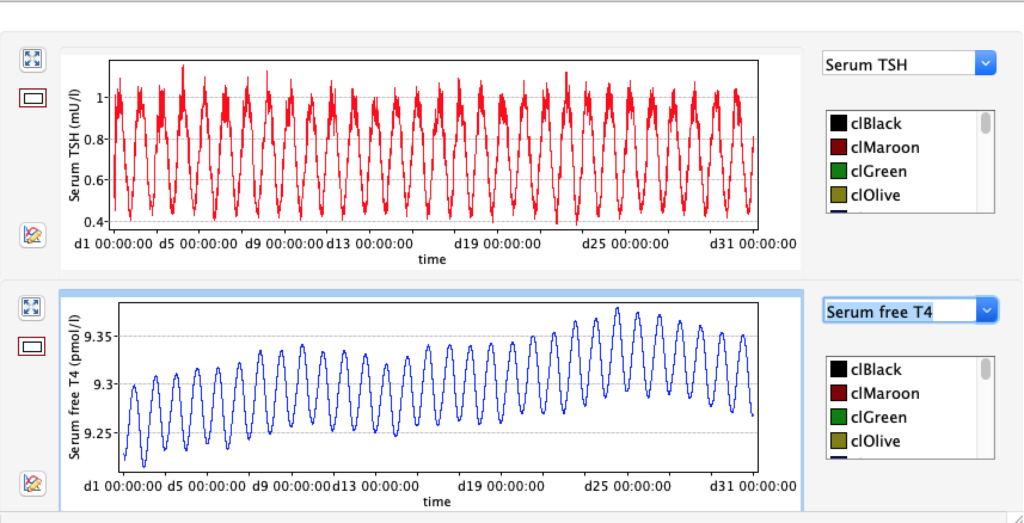
24 hour
In this TSH example you may see another trend in the development during the day – the height of the ridges changes as does the width
## Picking joint bandwidth of 0.0266
## Picking joint bandwidth of 0.0266

# Example of the code behind the the TRH plot
ggplot(CSVdotcsv, aes(x = TRH , y = as.factor(t), fill = as.factor(t))) + #as factor provides the legend for hour
#ggplot(CSVdotcsv, aes(x = TSH, y = t, group = t)) + # important to add group =
geom_density_ridges2(scale = 0.9) + #ridges 2 clearer to view
scale_y_discrete(expand = c(0, 0)) + # will generally have to set the `expand` option
scale_x_continuous(expand = c(0, 0)) + # for both axes to remove unneeded padding
coord_cartesian(clip = "off") + # to avoid clipping of the very top of the top ridgeline
theme_ridges() +
stat_density_ridges(quantile_lines = TRUE) +
labs( title = "TRH - 24 hours",caption = "J.W.Dietrich - SPINA package" ) +
scale_fill_cyclical(values = c("#4040B0", "#9090F0"))
## Picking joint bandwidth of 243
## Picking joint bandwidth of 243

Note that the echo = FALSE parameter was added to the code chunk to prevent printing of the R code that generated the plot.